Work with big data using Dask
Introduction
Working with large datasets can pose a few challenges - perhaps the most common is memory limitations on the user's machine.
Dask is a flexible, open source library for parallel and distributed computing in Python. Dask allows data scientists the ability able to scale analyses from a sample dataset to the full, large-scale dataset with almost no code changes. It's a powerful tool that can revolutionize how you do analytics!
Dask integration on Nebari
Nebari uses Dask Gateway to expose auto-scaling compute clusters automatically configured for the user, and it provides a secure way to managing Dask clusters.
Click here for quick notes on how Dask works!
Dask consists of 3 main components client, scheduler, and workers.
- The end users interact with the
client. - The
schedulertracks metrics and coordinates workers. - The
workershave the threads/processes that execute computations.
The client interacts with both scheduler (sends instructions) and workers (collects results).
Check out the Dask documentation and the Dask Gateway documentation for a full explanation.
Step 1 - Set up Dask Gateway
Let's start with a fresh Jupyter notebook.
Select an environment from the Select kernel dropdown menu
(located on the top right of your notebook).
On a default Nebari deployment, you can select the nebari-git-nebari-git-dask environment.
Be sure to select an environment which includes Dask, and note that the versions of dask, distributed, and dask-gateway must be the same.
We recommend the nebari-dask metapackage. We publish this metapackage alongside Nebari to easily provide you with the correct Dask packages and versions, just be sure that the nebari-dask version matches your Nebari deployment version.
If the nebari-dask environment does not include all the packages needed, here is a list to create a new environment:
- python >=3.11
- pip
- nebari-dask
- gcsfs
Nebari has set of pre-defined options for configuring the Dask profiles that we have access to. These can be accessed via Dask Gateway options.
from dask_gateway import Gateway
# instantiate dask gateway
gateway = Gateway()

# view the cluster options UI
options = gateway.cluster_options()
options
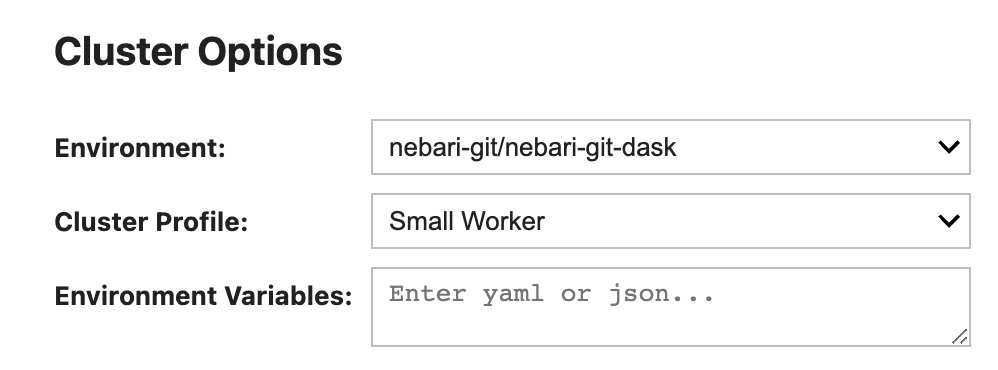
Using the Cluster Options interface, you can specify the conda environment for Dask workers, the instance type for the workers, and any additional
environment variables you'll need.
It’s important that the environment used for your notebook matches the Dask worker environment!
The Dask worker environment is specified in your deployment directory under /image/dask-worker/environment.yaml
The fields displayed in the Cluster Options UI are defined in the nebari-config.yml.
By default, you see "Environment", "Cluster Profile", and "Environment Variables", but you can configure this as per your (and your team's) needs.
Step 2 - Create a Dask cluster
-
Let's start by creating a new Dask cluster from within your notebook:
# create a new cluster with our options
cluster = gateway.new_cluster(options)
# view the cluster UI
cluster
Once you run the cell, you'll see the following:
-
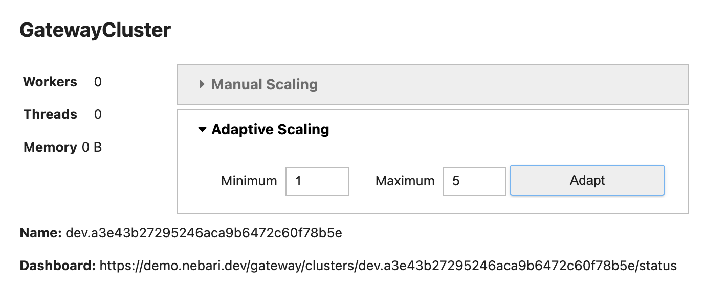
You have the option to choose between
Manual ScalingandAdaptive Scaling.If you know the resources that would be required for the computation, you can select
Manual Scalingand define a number of workers to spin up. These will remain in the cluster until it is shut down.Alternatively, if you aren't sure how many workers you'll need, or if parts of your workflow require more workers than others, you can select
Adaptive Scaling. Dask Gateway will automatically scale the number of workers (spinning up new workers or shutting down unused ones) depending on the computational border.Adaptive Scalingis a safe way to prevent running out of memory, while not burning excess resources.For this tutorial, we suggest trying the Adaptive Scaling feature. In the Gateway Cluster UI, set the minimum value to 1 worker and maximum to 5 workers, and click on the
Adaptbutton.You may also notice a link to the Dask Dashboard in this interface. We'll discuss this in a later section.
Step 3 - View the Dask Client
Once the Dask cluster has been created, you'll be able to get the cluster's information directly from your Jupyter notebook:
# get the client for the cluster
client = cluster.get_client()
# view the client UI
client
On executing the cell, you'll see the following:
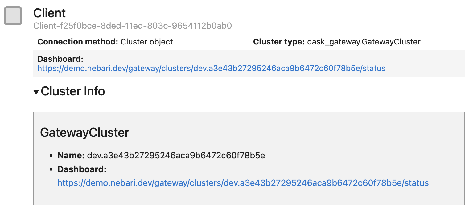
The Dask Client interface gives us a brief summary of everything we've set up so far.
Step 4 - Understand Dask's diagnostic tools
Dask comes with an inbuilt dashboard containing multiple plots and tables containing live information as the data gets processed.
To use the dashboard for the first time, click on the dashboard link displayed in the Client UI. This opens a familiar Keycloak authentication page, where you can sign-in the same way you authenticated into Nebari. Dask's browser-based dashboard opens automatically.
You can access the dashboard in two ways:
- Browser-based diagnostic dashboard
- Dask JupyterLab extension (recommended)
Dask's diagnostic dashboard will open in a new browser tab if you click on the dashboard links displayed in the Client UI or Cluster UI above.
The Dask-labextension is included with the default Nebari deployment. It provides a JupyterLab extension to manage Dask clusters, as well as embed Dask's dashboard plots directly into JupyterLab panes.
On JupyterLab, you can select the Dask icon in the left sidebar and click on the magnifying glass icon to view the list of available plots. Alternatively, you can copy-and-paste the dashboard link (displayed in the Client UI) in the input field.
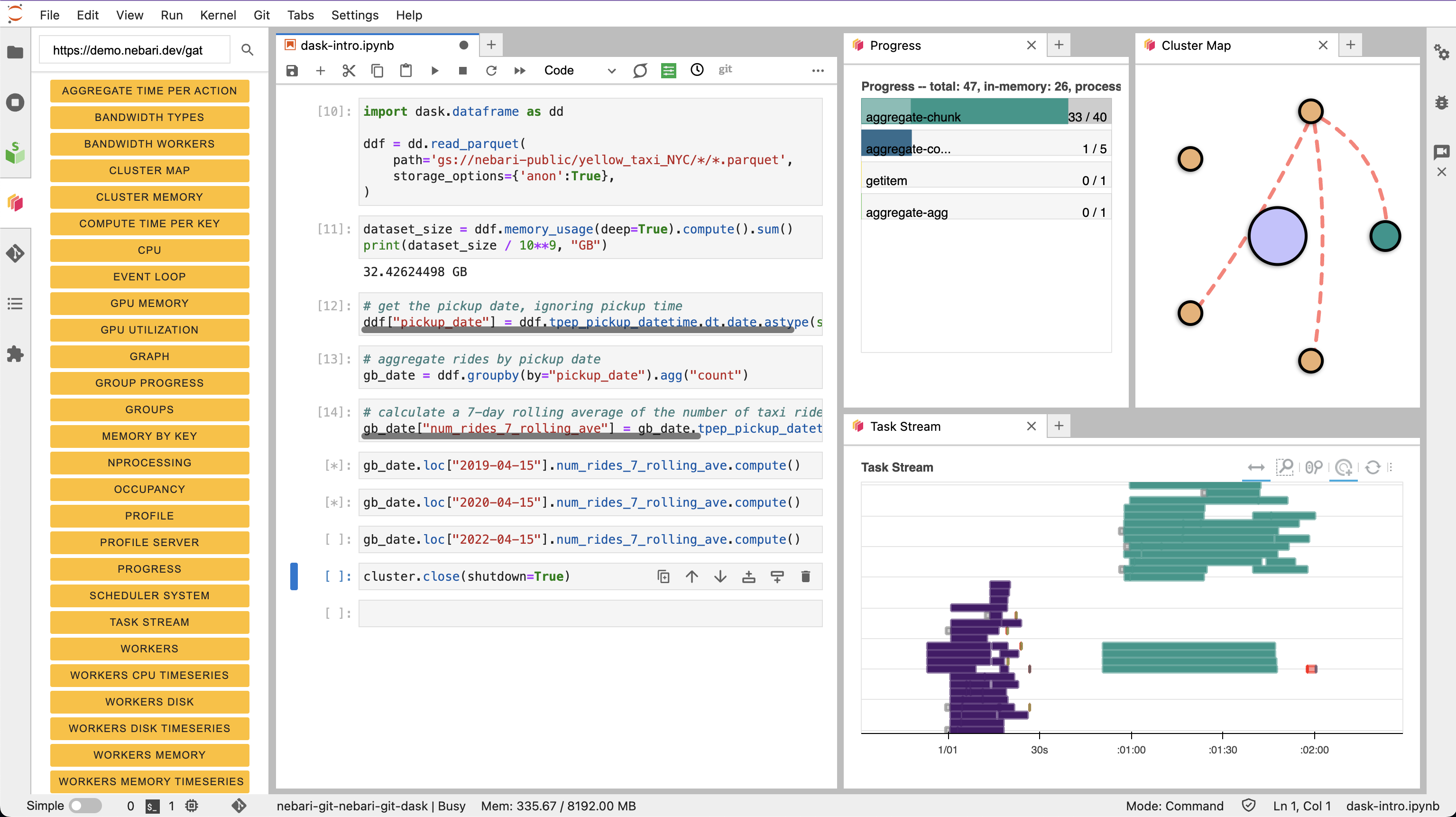
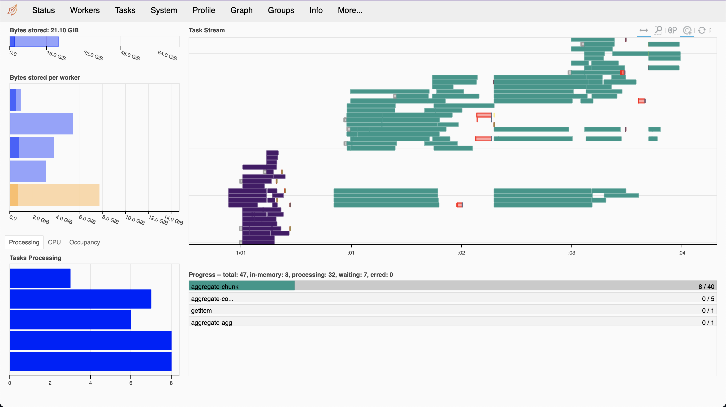
Let's open and understand the dashboard plots Task Stream, Progress, and Cluster map.
Most colors and the interpretation would differ based on the computation you choose. However, the colors remain consistent and represent the same task across all plots within the dashboard. Note that some colors always have the same meaning. For example, red always indicates inter-worker communication and data transfer.
Each of the computations you submit to Dask (you will learn more in the next section) is split into multiple tasks for parallel execution.
In the Progress plot, the distinct colors are associated with different tasks to complete the overall computation.
In the Task Stream (a streaming plot) each row represents a thread (a Dask worker can have multiple threads). The small rectangles within are the individual tasks running over time.
The Cluster Map shows the Dask scheduler at the center in a purple circle, with the active Dask workers around it in yellow circles.
This diagram is a convenient way to visualize Adaptive Scaling, and ensure new workers are being spun-up and shut-down based on workflow demand.
Check out the Dask Documentation on the dashboard plots for more information. Keep the dashboard plots open for the following computations!
Step 5 - Run your computation with Dask
In the following sections, you will perform some basic analysis on the well-known New York City yellow taxi dataset,
a subset of which we have copied over to a Google Cloud Storage bucket gs://nebari-public/yellow_taxi_NYC.
This dataset is saved in Parquet format, a column-oriented file format commonly used for large datasets saved in the cloud.
-
To get started, we will load the data using Dask's Dask DataFrame API. The following will lazily load the dataset::
import dask.dataframe as dd

ddf = dd.read_parquet(
    path='gs://nebari-public/yellow_taxi_NYC/*/*.parquet',
    storage_options={'anon':True},
) -
From here you can start analyzing the data. First, let's check the size of the overall dataset:
dataset_size = ddf.memory_usage(deep=True).compute().sum()
print(dataset_size / 10**9, "GB")
Output:
32.42624498 GBThis corresponds to 32.43 GB of data. Running this one-liner would be impossible on most single machines but running this on a Dask cluster with 4 workers, this can be calculated in under a minute.
-
Now, let's perform some actual analysis! We can for example, compare the number of taxi rides from before, during and after the COVID-19 pandemic. To do this, you'll need to aggregate the number of rides per day, calculate a 7-day rolling average and then compare these numbers for the same day (April 15th) across three different years, 2019, 2020, and 2022:
# get the pickup date, ignoring pickup time
ddf["pickup_date"] = ddf.tpep_pickup_datetime.dt.date.astype(str)
# aggregate rides by pickup date
gb_date = ddf.groupby(by="pickup_date").agg("count")
# calculate a 7-day rolling average of the number of taxi rides
gb_date["num_rides_7_rolling_ave"] = gb_date.tpep_pickup_datetime.rolling(7).mean() -
Now you can compare number of taxi rides on April 15th across three different years. In the
Cluster Map, notice how new workers are spun-up to execute that task.For April 15th, 2019 - pre-pandemic
gb_date.loc["2019-04-15"].num_rides_7_rolling_ave.compute()Output:
pickup_date
2019-04-15    259901.142857
Name: num_rides_7_rolling_ave, dtype: float64
or April 15th, 2020 - during the height of the pandemic
gb_date.loc["2020-04-15"].num_rides_7_rolling_ave.compute()Output:
pickup_date
2020-04-15    7161.857143
Name: num_rides_7_rolling_ave, dtype: float64
For April 15th, 2022 - post-pandemic
gb_date.loc["2022-04-15"].num_rides_7_rolling_ave.compute()Output:
pickup_date
2022-04-15    119405.142857
Name: num_rides_7_rolling_ave, dtype: float64
There were about 260,000 taxi rides a day in middle of April 2019 and that number plummeted to over 7,100 rides a year later, a full two orders of magnitude fewer riders. Wild!
Performing this kind of analysis on such a large dataset would not be possible without a tool like Dask. On Nebari, Dask comes out-of-the-box ready to help you handle these larger-than-memory (out-of-core) datasets.
Step 5 - Shutdown the cluster
As will you have noticed, you can spin up a lot of compute really quickly using Dask.
With great power comes great responsibility
Remember to shut down your cluster once you are done, otherwise this will be running in the background, and you might incur unplanned costs. You can do this from your Jupyter notebook:
cluster.close(shutdown=True)
Using Dask safely
If you're anything like us, we've forgotten to shut down our cluster a time or two. Wrapping the dask-gateway tasks in a
context manager is a great practice that ensures the cluster is fully shutdown once the task is complete!
Sample Dask context manager configuration
You can make use of a context manager to help you manager your clusters. It can be written once and included in your codebase. Here is a basic example to get you started (which can then be extended to suit your needs):
import os
import time
import dask.array as da
from contextlib import contextmanager

import dask
from distributed import Client
from dask_gateway import Gateway

@contextmanager
def dask_cluster(n_workers=2, worker_type="Small Worker", conda_env="nebari-git/nebari-git-dask"):
    try:
        gateway = Gateway()
        options = gateway.cluster_options()
        options.conda_environment = conda_env
        options.profile = worker_type
        print(f"Gateway: {gateway}")
        for key, value in options.items():
            print(f"{key} : {value}")

        cluster = gateway.new_cluster(options)
        client = Client(cluster)
        if os.getenv("JUPYTERHUB_SERVICE_PREFIX"):
            print(cluster.dashboard_link)

        cluster.scale(n_workers)
        client.wait_for_workers(1)

        yield client

    finally:
        cluster.close()
        client.close()
        del client
        del cluster
Now you can write your compute tasks inside the context manager and all the setup and teardown will be managed for you:
with dask_cluster() as client:
    x = da.random.random((10000, 10000), chunks=(1000, 1000))
    y = x + x.T
    z = y[::2, 5000:].mean(axis=1)
    result = z.compute()
    print(client.run(os.getpid))
Kudos, you should now have a working Dask cluster inside Nebari. Now go load up your own big data!